EYEGLASS: Adapting Computer Vision Models to Drifting Data with Foundation Model Finetuning

Developing computer vision models for tasks like object detection and activity recognition typically require a significant amount of human-curated labeled data. This issue continues after model development and into production, as additional human labeling is required to keep models up to date with drifting data and changing modeling objectives. 

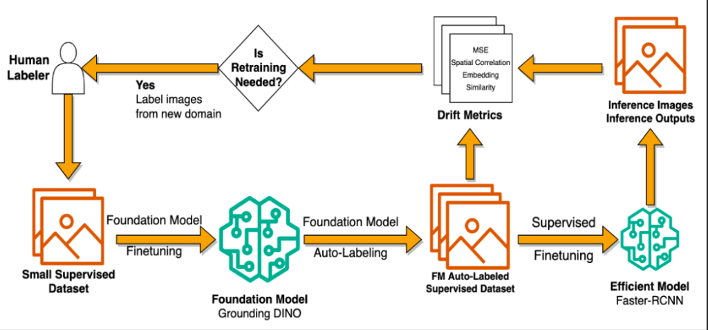
In this post, we outline the above model development pipeline, include our work studying auto-distillation methods, data drift detection, and model adaptation. We customize large pretrained foundation models and use them to train lightweight object detection models, increasing performance by 33% over human label only trained models, while running inference 20x faster. We also study metrics for identifying when to retrain models and apply this technique to finetuning models for new data and new modeling objectives.

The Auto-Distillation Process

Training robust computer vision models typically requires a large amount of human-labeled data. While techniques like transfer learning reduce the labeling burden, it can still take hundreds to thousands of images to develop a performant model. Human labeling is difficult and expensive in terms of human time and effort. This is increasingly true for highly domain-specific data – labelers must also be domain experts and pretrained backbones may offer less benefit on obscure and specific data sets. In order to minimize these issues, we utilize a process called auto-distillation to leverage large pretrained models to amplify the power of human labeling for training more performant models with less time and effort.

The auto-distillation process is not unique to this work. Services like Roboflow offer the capability to leverage large foundation models such as Grounding DINO and Segment Anything to generate labeled datasets for finetuning performant student models like YOLOv8. However, we expand on this process by introducing an initial foundation model finetuning step, enabling stronger distillation performance on domain specific datasets. We leverage a small set of human labels to fine-tune a foundation model, directly improving its labeling capabilities on our specific domain. Then, we proceed with the auto-distillation process, generating tens of thousands of annotations that we can use to train smaller, more performant models.

In practice, we found that foundation model annotation performance scaled with the number of human labels for our data and Faster-RCNN model training saturated around 10,000 images. By first finetuning our foundation model (Grounding DINO), we were able to increase performance of our student model (Faster-RCNN) on our evaluation set by 22% over a model distilled from a zero-shot foundation model. This student model was also 18% more performant than if the student model were only finetuned on the human labels used to finetune the foundation model, demonstrating the ability of foundation model finetuning to amplify the power of human labeling. 

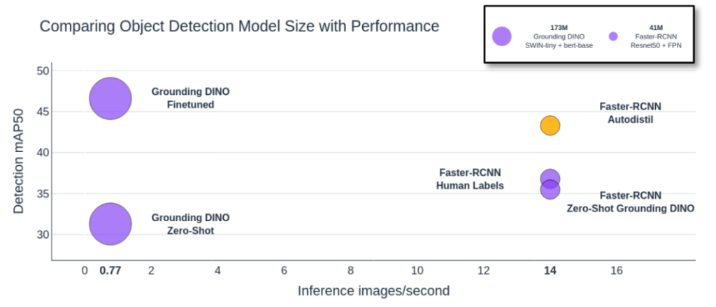
The chart above shows the impacts of finetuning foundation models as well as the impacts of distilling them into performant student models. Moving from zero-shot to finetuned Grounding DINO increases performance by 49%, while distilling Grounding DINO into a Resnet-50 Faster-RCNN model increases inference speed by almost 20x.

Identifying Data Drift

Now that we can train high performing, efficient computer vision models, we can deploy them into production. However, in production, we observe the performance of the models deteriorating over time. This is likely due to the data they are running on drifting from the data they were trained on. Missed detections or false positives can incur significant costs to the mission, so it is imperative that we can identify when these shifts occur and adapt to them appropriately.

First, let’s define two types of data drift – out of distribution and out of domain. Out of distribution data is similar to the training data, but is not exactly the training data, while out of domain data is categorically different than the training data. For example, if we train a model on images from Midway Airport like the one below, we might say images from St. Barth airport are in domain, but out of distribution. In contrast, the street-view of a bus from COCO would be out of domain and out of distribution, because it is distinctly different than anything in the training data. 

Figure 4: Examples of Distribution and Domain Shift

The question then becomes – how can we detect these types of data drift? To do this effectively, we need to be able to:

1. Quantify how different inference data is from training data
2. Predict changes in model performance based on differences in the inference data
3. Run the drift detection efficiently across a large amount of training and inference data

We compared three datasets to the data that a model was trained on:

Dataset	Description	In Distribution?		In Domain?
Baseline Test	Model test set – same airports as training	✅	✅
New Feeds	Images from airports not used to develop the model	✅	❌
Out of Domain	Images not of airports, from the COCO dataset	❌	❌

Between each of these datasets and the training dataset, we computed 21 metrics, split between pairwise and image-level metrics. Pairwise metrics were computed between each image in the training data and each image in each of the 3 datasets. Examples of pairwise metrics are mean-square-error (MSE), structural image similarity (SSIM), and the spatial correlation coefficient (SCC). Image metrics were computed per image and differenced between each dataset and the training data and include mean pixel value, image saturation, and image brightness. For each metric, we calculated the extrema (min/max) to evaluate the closest point to the training data. Additionally, we tracked the per-image object detection performance (mAP@50) and the per-image average model confidence scores. 

We studied the relationship between all 21 image metrics plus the model confidence scores and object detection performance. We found that several metrics saw drastic change between the baseline, new, and out of domain datasets.

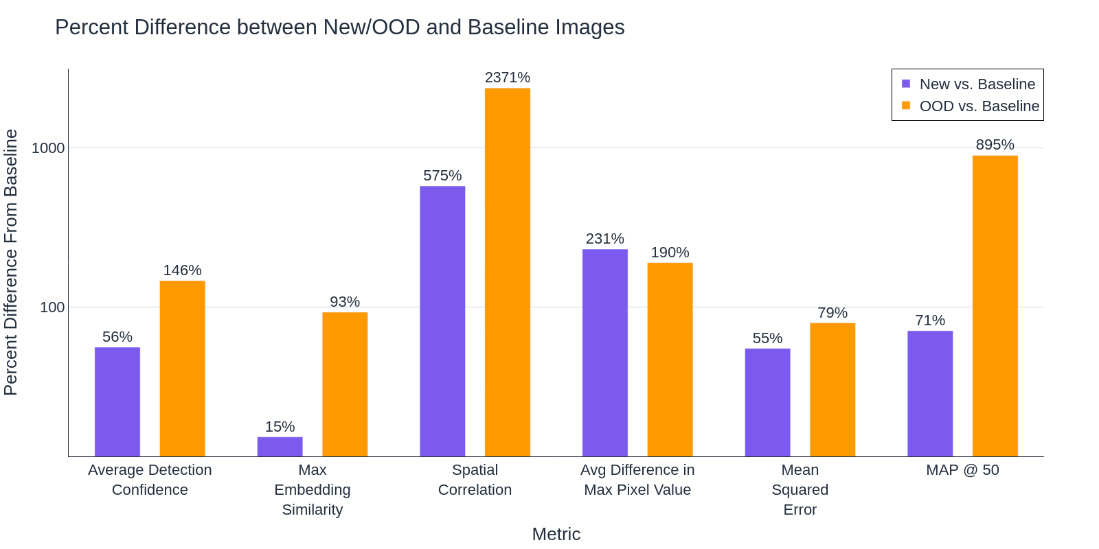
Clearly, object detection performance (MAP @ 50) changes significantly as the data drifts further away from the training data. Some metrics, like MSE and Average Pixel difference, saw large changes from the baseline in both datasets, while others like Max Embedding Similarity and Spatial Correlation, are better equipped to separate in-domain and out-of-distribution data.

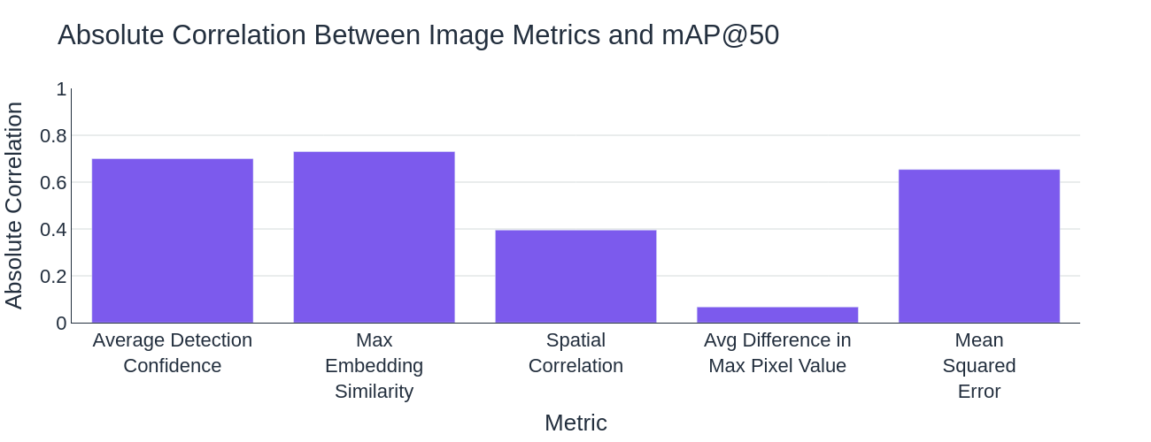
We also looked at the linear correlation between these metrics and detection performance, finding detection confidence and embedding similarity to be strongly correlated. This leads us to believe that these metrics may be used as strong predictors of detection performance. 

Many of these metrics satisfy our first two requirements, they quantify the difference between images and can be used to predict reduced detection performance, but what about being efficient to calculate? Between pairwise metrics, image metrics, embedding similarity, and detection confidence, they each have their own tradeoffs in terms of the cost of the computation and the number of computations that need to be made.

Figure 7: Compute Cost vs. the Number of Computations for Drift Detection Metrics

Overall, we found that several metrics are suitable for identifying changes in the distribution and domain of inference data. We found detection confidence, embedding similarity, and the spatial correlation coefficient to be the most reliable, but even mean square error can be a reasonable predictor. If you are trying to prevent spending expensive compute, use the simpler to calculate image similarity metrics. If running models on drifting data is less of a concern, detection confidence and embedding similarity may be better options.

Adapting to Data Drift

After identifying a change in the data’s distribution, it becomes necessary to update the inference model to maintain performance. However, it is not obvious how best to do this – should the model be fine-tuned or retrained? What data should be used? Can the distillation process aid adaptation?    

To answer these questions, we compare multiple data-centric adaptation methods.  We first train a model using the standard distillation process on images from a specific set of airport feeds and then adapt it to images from a new set of feeds. We compare the following methods for adapting the model, seeking to maximize performance on new data and prevent catastrophic forgetting of original, baseline data:

1. Fine-tune a model pretrained on baseline data with hand-labeled images from new feeds
2. Fine-tune a model pretrained on baseline data with auto-labeled images from new feeds
3. Fine-tune a model pretrained on baseline data with a mix of auto-labeled images from new feeds and original training data. 
4. Fine-tune a model pretrained on ImageNet with a mix of auto-labeled images from new feeds and original training data.

For each method, we assess performance on both original data and new feed data relative to the original model.  Results are in Figure 8.

Figure 8: Comparison of methods for adapting to new feeds 

Fine-tuning Grounding DINO with hundreds of hand-labeled images from new feeds, using it to auto-labeling thousands more and then tuning the original model with the auto-labeled images outperforms tuning the original model directly with hand-labeled images.  This suggests that the distillation pipeline is useful not only for training an initial model, but adapting it to changing data conditions as well.  Additionally, we find that including original training data in the fine-tuning prevents catastrophic forgetting. The best overall performing model was fine-tuned in this way with a mix of original training data and auto-labeled new data.  Finally, we see that fine-tuning a model pretrained on baseline data achieves better performance than fine-tuning a model pretrained on ImageNet with the same data. 

Another common reason to adapt an inference model is the addition of a new class. We investigate this in a similar manner to above, by training a baseline model to recognize a fixed set of classes and adapting it with images that contain a new class. Figure 9 displays the overall and new class performance relative to the baseline model for each adaptation method.

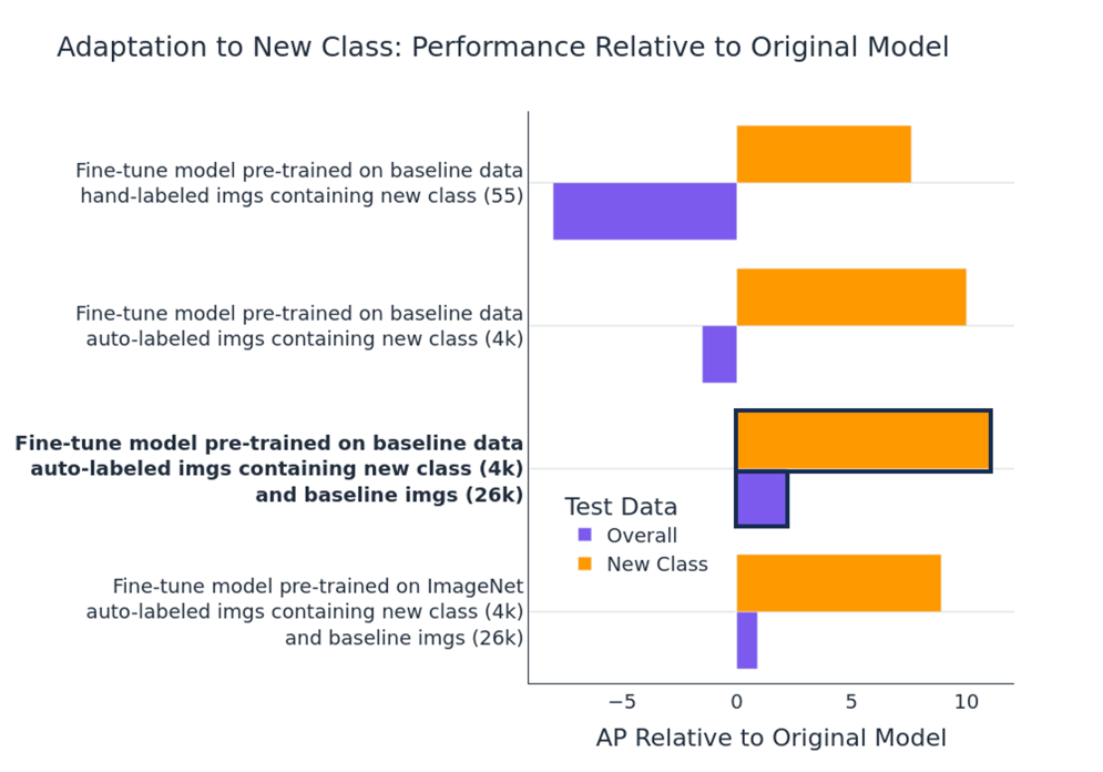
The results are analogous to those above. Fine-tuning with a mix of original data and auto-labeled images with the new class is the optimal method for adapting the model. The inclusion of original images helps to prevent catastrophic forgetting.

Oftentimes, thousands of examples of the new class are unavailable for auto-labeling.  In this case the model can be adapted with small-scale tuning of just the detection head. (We tuned with a partially frozen backbone in previous experiments.) With just 50 images of the new class along with a few hundred original images, a majority of data-rich new class performance can be achieved with minimal overall performance drop off (Figure 10). 

	Original Images	New Class Images		Overall AP	New Class AP
Baseline model	26k	0	21		0
Data rich fine-tuning	26k	4k	23.2		11
Few-shot fine-tuning	444	50	19.6		10.7

Conclusion

In this work, we developed a model development pipeline capable of training performant object detection models and adapting those models to drifting data with reduced human effort. By leveraging large foundation models, we are able to synthetically augment human labels and shift compute from inference time to training time. This results in models that are not only more efficient than their foundational teachers, but are more performant than those trained on human labels alone. Our research points to multiple metrics that enable us to identify when our target data is changing and proposes performant model adaption methods without catastrophic forgetting.

Contact Info

• Sam Saltwick (saltwick@amazon.com)
• Kyle Rose (kymrose@amazon.com)
• Will Gleave (sgleave@amazon.com)
• Julie Hong (hongjth@amazon.com)

This material is based upon work done, in whole or in part, in coordination with the Department of Defense (DoD). Any opinions, findings, conclusions, or recommendations expressed in this material are those of the author(s) and do not necessarily reflect the views of the DoD and/or any agency or entity of the United States Government.